Markdown tables in LaTeX
LaTeX is a fantastic way to create and display print-ready scientific documents. There are a number of different ways to edit and produce LaTeX documents, which we’ll revist in a future post. In this post, I want to deal with one of the major issues that people find difficult with LaTeX: tables.
LaTeX can certainly produce any type of table you’d like to create, but it does so in a way that can be very difficult to follow visually.
For example to produce the following table, we’d use this code:
\begin{table}[]
\begin{tabular}{|c|c|}
\hline X & P(X = i) \T \\\hline
  1 \T & 1/6 \\\hline
  2 \T & 1/6 \\\hline
  3 \T & 1/6 \\\hline
  4 \T & 1/6 \\\hline
  5 \T & 1/6 \\\hline
  6 \T & 1/6 \\\hline
\end{tabular}
\end{table}
which produces output like this:
$$\newcommand\T{\Rule{0pt}{1em}{.3em}} \begin{array}{|c|c|} \hline X & P(X = i) \T \\\hline 1 \T & 1/6 \\\hline 2 \T & 1/6 \\\hline 3 \T & 1/6 \\\hline 4 \T & 1/6 \\\hline 5 \T & 1/6 \\\hline 6 \T & 1/6 \\\hline \end{array}$$
One way to make producing LaTeX tables easier is to use a graphical generator, for instance Tables Generator. However, this doesn’t really help when you have to go back and edit tables. It can be very difficult to find a place in the syntax especially when cell contents have variable sizes.
Using knitr to process markdown tables
I was interested in seeing if I could bring some richer features to table editing in LaTeX by using the excellent package knitr to allow the use of R in LaTeX. The idea was to write tables in markdown format, process them using R and output them using xtables back to the LaTeX document. This sounds complicated but once you have the glue written, it simplified table handling enourmously and also permits very useful manipulations like table arithmetic.
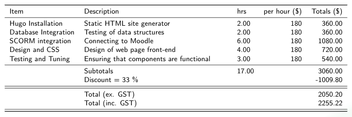
Here’s an example of what we may do for a price quote for instance:
Markdown Table
Create a markdown table and save it as table.md
Item                 | Description                              | hrs   | rate
---------------------|------------------------------------------|-------|----
Hugo Installation    | Static HTML site generator               | 2     | 180
Database Integration | Testing of data structures               | 2     | 180
SCORM integration    | Connecting to Moodle                     | 6     | 180
Design and CSS       | Design of web page front-end             | 4     | 180
Testing and Tuning   | Ensuring that components are functional  | 3     | 180
                     | Subtotals                                |       |
                     | Discount                                 |       |
                     | Total (ex. GST)                          |       |
                     | Total (inc. GST)                         |       |
Markdown tables are easy to read and edit and can be rendered into other formats easily. Notice in the table above that we’ve left some fields blank, we’re going to use R to process these fields.
knitr
We can do this by creating a table_build.knitr file which we will then call from the LaTeX document.
<<table_1, echo=FALSE, results="asis", cache=FALSE>>=

tablename="table.md"

headers<-read.table(tablename, sep = "|", header=TRUE, nrows=1)
table<-read.table(tablename, sep = "|", skip=1, header=TRUE)
colnames(table) = colnames(headers)

# set as character rather than factor
table$Description<-as.character(table$Description)

# calculations
# by-row totals
table$totals<-table$hrs * table$rate

# subtotals
table$hrs[nrow(table)-3]<-sum(table$hrs, na.rm = T)
table$totals[nrow(table)-3]<-sum(table$totals, na.rm = T)

# Discount calculation and input
discount = 0.33
table$Description[nrow(table)-2] <- paste("Discount = ", (discount*100)," \\%",sep="")
table$totals[nrow(table)-2] <- table$totals[nrow(table)-3]*(-discount)

# column totals - to be filled in to the last row
table$totals[nrow(table)-1]<-table$totals[nrow(table)-3]+table$totals[nrow(table)-2]
table$totals[nrow(table)]<-table$totals[nrow(table)-1]*1.1

colnames(table)[4] <- "per hour (\\$)"
#colnames(table)[3] <- "\\textbf{test}"
colnames(table)[5] <- "Totals (\\$)"

library(xtable)
options(xtable.sanitize.rownames.function=identity)
options(xtable.sanitize.colnames.function=identity)
options(xtable.sanitize.text.function=identity)
tab <- xtable(table)
align(tab) <- "llXlrr"
hlines <- c(-1, 0, nrow(tab),nrow(tab),(nrow(tab)-2),(nrow(tab)-2),(nrow(tab)-4))
print(tab, type="latex", include.rownames=FALSE, booktabs=T, floating=FALSE, tabular.environment="tabularx", width = "\\textwidth",
hline.after = hlines)
@
This R script pulls in the markdown file and reads it as tabular data, it then does some calculations and inserts totals and calculated discounts. The script could be altered to do a number of calculations or more advanced logic.
The R script can also be reused on multiple tables. Note that we’ve used the booktabs and tabularx packages to format the table.
Output
Integration into LaTeX document
To use knitr in LaTeX, you’ll first of all need to have R installed on your computer and allow shell execution permission to your LaTeX compiler.
Then it’s a fairly simple matter of renaming your LaTeX file to an .Rtex file so that the interpreter knows to expect knitr code chunks.
Then we just add the following:
Preamble:
\usepackage{booktabs}
\usepackage{tabularx}
In main document:
% table.md
<<call_table, child="tables/table_build.knitr">>=
@
Conclusion
Now we can easily use markdown-style formatted tables in LaTeX documents and also do calculations with these tables. Some of you may be thinking that we’ve really just moved the complexity from the LaTeX table to the knitr R script, but I think this is worth the effort as the tables are now much easier to maintain and edit. Hopefully is follows the idea of “write once, use many times”. As always, I’m interested to hear your comments.